
Introduction
Nowadays data has become “The One Ring”. Every single decision has to be taken with the most updated available information and it has reached basically every single industry. Movies do a small screening test for a select audience to gather information and see which parts are the most and least liked ones. Tech companies gather data around their sold products to see which ones are bought the most. Even us, regular people, use data from other people to choose the best restaurant based on online reviews.
Whether the use of this data is meaningful, conclusive or correctly applied usually doesn’t come into effect until the product has already been launched or simply some time has passed. This is what we can call an “a posteriori” usage of the data. We let the things flow their way, we recompile the information and we improve for future iterations. However, there are certain cases where this workflow doesn’t make complete sense, and where this precious treasure we call data should be used in a different way.
What if we know about an incoming storm, let things flow, gather the information afterwards and improve for the next time it happens? In theory it makes sense, but no two storms are the same. Similar? Perhaps. There is no guarantee that lightning will hit twice on the same spot, so focusing on just the previous event might lead to false assumptions. We can however, learn from all previous storms, generalize trends and behaviours, identify the most critical points and use this information to our advantage. Prevent and prevail. We use this gathered data “a priori”, to avoid future disasters and help manage a situation that could get way worse and out of hand easily.
A good example of this usage could be applied to batteries. Almost everyone that has ever had a phone or a computer is familiar with the feeling of knowing the battery keeps getting worse and worse and not being able to do anything about it, until one day it inevitably stops working. Some people are precocious, and might find a replacement with enough time. Others, however, wait for too long and now everything saved on their device is gone forever. Wouldn’t it be useful to know in advance how bad the health of a certain battery is? This is more or less the objective of this blogpost. Is there any way we can predict the life cycle of a battery and use that information to our advantage?
Battery data & Testing process
Before we can start thinking about saving the life of any device with a battery, let's first define what we mean by the life cycle of a battery and how it applies to the specific dataset used for this experiment.
If there is no information available, life cycle could mean many different things: The life of a battery (in days, months, years,...) from the day it is made to the day it stops working, It could also mean the information that is received from the battery every X minutes, hours, days, … until the death of it. However, for this concrete dataset, the life cycle refers to the charge-discharge cycle number of any battery. In other words, for this dataset, a series of lithium batteries were fully charged and artificially discharged. One full charge into a complete discharge counts as one cycle. In addition to charging cycles, the dataset also includes information about:
- battery_id: Unique identifier for each battery cell
- cycle: Current cycle of the battery
- IR: Internal resistance of the battery
- QC: Charge capacity during charging
- QD: Discharge capacity during discharging
- Tavg: Average temperature during the cycle
- Tmin: Minimum temperature during the cycle
- Tmax: Maximum temperature during the cycle
- chargetime: Time required to complete charging
- C1: First charging rate extracted from charging policy
- Q1: Percentage at which charging rate changes
- C2: Second charging rate extracted from charging policy
- RUL: (Rest of Usable Life) Total life-cycle of the battery (cycles until end-of-life)

It is important to note that this dataset was cleaned and prepared prior to its upload to Kaggle, so most of the hard work necessary to make the data ready is skipped. Once we have all the necessary correct data, the next step is to make our training/test splits for our ML algorithms. The complete file contains 140 different batteries with varying amounts of life cycle values. For this experiment, 112 batteries (80%) were used on the training set, while 14 (10%) batteries were used in both the validation set and test set.
Another very important decision related to the different sets is how the whole Machine Learning pipeline will work. But first, let's define the purpose of this project. There are two main objectives we would like to achieve. The first one is pretty obvious, we want to predict the RUL of a battery when we only have part of the battery’s information. For the second part, however, we want to predict the values of the non-stationary variables for each cycle until the predicted end of life cycle. These values include IR, QC, QD, Tavg, Tmin, Tmax and chargetime.
In either case, the available information for the predictions is limited, so we have to train our ML algorithm carefully. We will use two different setups that share a very similar pipeline and differ only in what the model is asked to predict. In both, the model never sees a battery’s full history at once. Instead, each battery is cut into windows of 30 consecutive cycles, and the model learns to make a prediction from one window. For the training and validation sets, every possible window is used: a window ending at cycle 30, another ending at cycle 31, and so on until the end of the battery’s life. This turns the 112 training batteries into a large number of examples, from early life up to end of life. Each window contains the seven measured variables (IR, QC, QD, Tavg, Tmin, Tmax and chargetime) for its 30 cycles. All values are scaled by dividing each variable by its largest absolute value in the training set. The validation and test sets are scaled with these same training values, so no information from them leaks into training.
The difference between the two objectives lies in the target. When predicting the RUL, the target is a single value: the RUL at the last cycle of the window, that is, how many cycles the battery has left after the 30 cycles the model has seen. The RUL is used only as the answer during training and is never given to the model as an input, since it depends on the battery’s end of life, which is unknown at prediction time. When predicting one of the other variables, the target is that variable’s value for each of the next 30 cycles after the window, so the model produces 30 values at once. In this case the past values of the variable are allowed as inputs, because only its future values are being predicted. For example, the chargetime of the last 30 cycles helps predict the chargetime of the next 30. Since these windows need 30 known cycles after them, the last 30 cycles of each battery cannot be used as a window end in this setup.
Testing is done on the 14 test batteries, which the model has never seen during training or validation. To evaluate how the model performs at different points of a battery’s life, each test battery is divided into three equal parts: early, middle and late life. A window is assigned to a stage according to the cycle where it ends, which is the moment the prediction is made. Two windows are then chosen at random from each stage of each battery, which gives 6 windows per battery and 84 test windows in total. The model receives only 30 cycles of input variables of each window. The true values are kept aside and used only afterwards to score the predictions. The results are converted back to their original units and evaluated with the mean absolute error (MAE), the root mean squared error (RMSE) and the coefficient of determination (R²). These are computed for the whole test set and separately for each life stage.
In this process, there are many decisions that were taken without much argument and could perfectly be modified based on more evidence or knowledge. For example:
- Using the previous 30 cycles to predict the next one.
- How far ahead we want to predict values.
- The importance given to every cycle of the window
- Usually later cycles are more important than older ones.
It is also important to note that predicting values continuously after a certain threshold without some correcting will most likely lead to either predictions being just the mean/average of the values or some extreme values. One way to fix this issue is using real values to correct the trajectory. Once we get the real data from the 31st cycle, we inject it to the model so it can calculate errors and adjust, instead of just predicting even more far ahead.
ML models & results
Now that we have decided on our data, our objectives and our outputs, we need the tools to reach those objectives. We use two different algorithms: XGBoost (eXtreme Gradient Boosting) and a GRU (Gated Recurrent Unit), a type of recurrent neural network. XGBoost is used only for the first objective, predicting the RUL. The GRU is used for both objectives: predicting the RUL and forecasting the battery’s measurements. Both algorithms use exactly the same data: the same training, validation and test batteries, the same 30-cycle windows and the same test windows. Their results can therefore be compared directly.
XGBoost works by building an ensemble of small decision trees sequentially, with each new tree trained to correct the prediction errors (residuals) of the previous ones.
The Core Boosting Process
- Base prediction: The model starts with a simple initial guess for every data point, such as the average value of the target.
- Calculate errors: It calculates the residuals, which measure the gap between the current predictions and the true values.
- Build a new tree: A new decision tree is built to predict these errors from the input features. It searches for the splits that best group data points with similar errors together. Each leaf then outputs a correction value, which is essentially the average error of the points in that leaf, pulled slightly towards zero by regularization.
- Shrink and add: The output of the new tree is scaled down by a learning rate (step size) to keep the model stable, and added to the cumulative prediction.
- Repeat: The process repeats for up to 1,000 trees, or until the error on the validation batteries has not improved for 50 consecutive trees, steadily shrinking the remaining errors. The model then keeps the number of trees that gave the lowest validation error.
Example
Step 1: Summarising each window. XGBoost requires a flat, two-dimensional table: one row per sample and one column per feature. It cannot read a sequence of cycles the way a GRU does. Each 30-cycle window is therefore summarised before it is given to the model. For each of the 7 measured variables (IR, QC, QD, Tavg, Tmin, Tmax and chargetime), six numbers are computed over the window: the last value, the mean, the standard deviation, the minimum, the maximum and the slope (how fast the variable is changing per cycle). Each window thus becomes one row of 42 columns (7 variables × 6 statistics), with names such as QD_slope or IR_last. The slope columns are what give the trees a sense of trend: they tell the model not only where a variable is, but in which direction it is moving.
Step 2: Base prediction and initial errors. Before building any trees, the model sets one baseline guess for all windows. Let’s assume the average RUL of the training windows is 300 cycles. It then calculates the initial residual (error) for each window:
- Window A residual: 450 (true) − 300 (guess) = +150 (model underpredicted)
- Window B residual: 210 (true) − 300 (guess) = −90 (model overpredicted)
Step 3: Building Tree 1 (targeting the errors). Tree 1 goes through all 42 columns, testing possible split points in each, and picks the split that best separates the windows according to their errors. Suppose the cleanest grouping comes from QD_slope, the rate at which the discharge capacity is falling over the window:
- Leaf 1 (capacity falling slowly): predicts +100 (fits window A, a healthy battery with a long life ahead)
- Leaf 2 (capacity falling quickly): predicts −60 (fits window B, a battery that is degrading fast)
Step 4: Shrink and add. To keep the model stable and prevent it from overfitting to the first tree, XGBoost scales the tree’s output by the learning rate (0.05 in our model):
New prediction = old prediction + (0.05 × tree output)
- Window A updated prediction: 300 + (0.05 × 100) = 305
- Window B updated prediction: 300 + (0.05 × −60) = 297
Step 5: Repeat. The algorithm calculates the new, slightly smaller residuals based on the updated predictions:
- Window A new residual: 450 − 305 = +145
- Window B new residual: 210 − 297 = −87
Tree 2 is then built to target these updated residuals. This loop runs for hundreds of rounds, with each new tree moving the predictions a little closer to the true values.
A few things to keep in mind
- Tree depth is a tunable hyperparameter. Our example tree has a single split, but the trees in our model can be up to 6 levels deep. A tree of depth d can have up to 2^d leaves, so deeper trees capture more complex interactions between features, at a higher risk of overfitting.
- Overfitting is easy. Consecutive windows of the same battery are very similar, so the trees can end up memorising the training batteries. To counter this, each tree is built on a random 80% of the training windows and a random 80% of the columns. Together with the low learning rate and early stopping on the validation batteries, this keeps the model general.
- Extreme values are hard to predict. Each leaf outputs a value based on the training samples that fall into it, so the model cannot predict beyond the range it saw during training. Batteries with unusually long or short lifetimes tend to be pulled towards more typical values. Predictions are also limited to zero or more, since a negative RUL is impossible.
The Core Recurrent Process (GRU)
For the GRU part of the project, we train separate models, each for its own task:
- The RUL GRU predicts the battery’s remaining useful life (RUL) directly, so it tackles the same task as XGBoost.
- The forecasting GRUs predict how one of the battery’s measurements will evolve over the next 30 cycles. One model is trained per variable, for example one for chargetime and one for QC.
All of these models have the same architecture, read the data in the same way and are trained in the same way. They differ only in what they are trained to output.
How the GRUs read the data
- Sequential processing: XGBoost sees each window as one row of summary numbers. A GRU instead steps through the 30 cycles of the window in order, one cycle at a time.
- Hidden state (memory): As it moves from cycle to cycle, the model keeps a hidden state, a running numerical summary of the battery’s behaviour so far.
- Gating mechanism: At each step, the model uses learned filters called gates to manage this memory. The update gate decides how much of the old memory to keep and how much to replace with information from the new cycle. The reset gate decides how much of the past memory to use when interpreting the new cycle, so the model can ignore history that is no longer relevant.
Where the GRUs differ
- RUL GRU: After reading the window, it turns its final hidden state into a single number: the RUL. One window in, one RUL out. The RUL is only used as the answer during training. It is never given to the model as an input, because it depends on the battery’s end of life, which is unknown at prediction time.
- Forecasting GRU: After reading the window, it turns its final hidden state into 30 values: the predicted value of its variable for each of the next 30 cycles. Here, the past values of the variable being forecast are allowed as inputs. For example, the chargetime of the last 30 cycles helps predict the chargetime of the next 30, because only its future values are being predicted.
The rest of this section focuses on the RUL GRU.
Example (RUL GRU)
Step 1: The GRU reads the first cycle of the window: 7 measurements. These values first pass through an input layer, which transforms them into a richer internal description of the cycle. The GRU layer uses this description to start its hidden state. It then moves to the second cycle and updates its memory by combining what it learned from the first cycle with the new measurements. It repeats this up to the 30th cycle, building a summary of how the battery is behaving over the window. Several GRU layers can be stacked, each reading the output of the one before it. This lets the deeper layers pick up more complex patterns, such as how fast the battery is degrading rather than just how degraded it is.
Step 2: After the 30th cycle, the final hidden state passes through a few dense layers that turn the GRU’s summary into the prediction. Dropout is applied during training to reduce overfitting. The last layer uses a softplus activation, which keeps the prediction positive. The result is just one value: the predicted RUL at the last cycle of the window, meaning how many cycles the battery has left from that point.
Step 3: RUL ranges from a few cycles to about 2,000, so the model does not learn the raw number. Before training, the RUL is divided by the largest RUL in the training set, which puts every target between 0 and 1. The 7 input variables are scaled in the same way, each by its own largest training value. The model’s output is then multiplied back by the same factor to give the RUL in cycles. The scaling factors come from the training set only, so no information from the validation or test batteries leaks into the model.
We build two different GRU models (a smaller one and a bigger one) and a XGBoost model to predict the RUL. In the following tables we can see the comparison on the results between them.
Here, the MAE is the average number of cycles by which the predicted RUL differs from the true RUL. The RMSE penalises large errors more, so it shows whether a model makes occasional big mistakes. R² is the share of the variation in the true RUL that the model explains, where 1 is perfect and 0 is no better than always predicting the average. XGBoost performs best on all three metrics, with an MAE of 62 cycles, compared with 100 cycles for the large GRU and 131 for the small one.
The second table shows the same metrics for each of the three life stages. All models improve significantly from the early to the late life of a battery, and XGBoost remains the most accurate in every stage. Early in life, the batteries show few signs of degradation, which makes the RUL much harder to predict. Late in life, the degradation is clearly visible in the measurements.
The table above shows six test windows chosen at random (two from each life stage) together with the predictions of each model.
Error bias
Looking at the bias of the errors, both GRU models tend to overpredict the RUL on average, while XGBoost tends to underpredict it. Underprediction is the safer tendency: it means the model expects a battery to fail slightly earlier than it actually does.
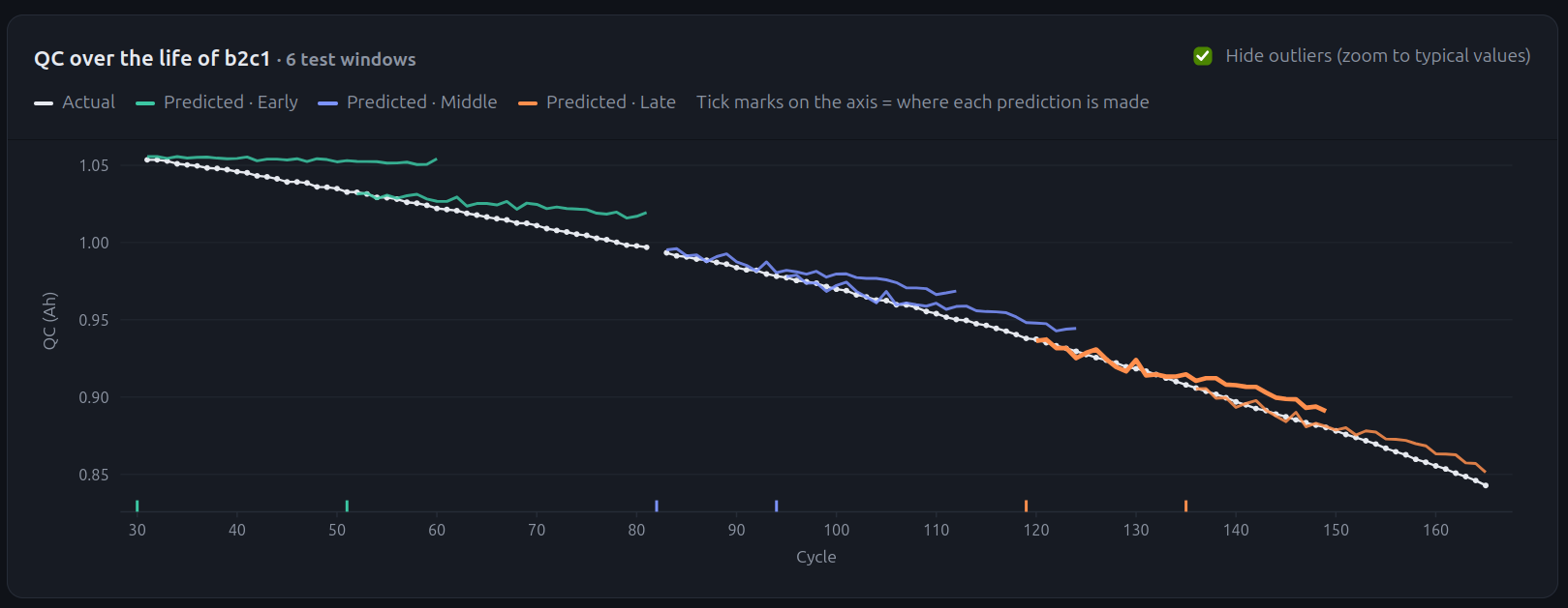
We also trained a model that predicts the QC of a battery for each of the next 30 cycles, using only the previous 30 cycles. Some of its results can be seen in the following graph.
Conclusion
So, can we predict the life cycle of a battery? To a good extent, yes. Using only 30 cycles of measurements, our best model, XGBoost, predicted the remaining useful life with an average error of about 62 cycles and explained over 93% of its variation. It also tended to slightly underestimate the remaining life, which is the safer mistake when the goal is to replace a battery in time. Predictions become much more accurate as the battery ages, precisely when they matter most, while early life remains the hardest stage to read, since degradation has barely started. Forecasting the measurements themselves, such as the charge capacity over the next 30 cycles, also proved feasible. There is still room for improvement: we could revisit decisions like the window length and the prediction horizon, or feed real measurements back into the model to correct its trajectory. Even so, the results show that data does not have to be used only a posteriori. Used a priori, it can warn us about the storm before it arrives, and give us the chance to save our data before the battery gives up.